
Elections are the most important events of political life. Their results determine who gets to be in government for the next few years. But how long do elections and their results capture the public's attention? In this blog post we take a look at Wikipedia page access statistics to find out.
Our weapon of choice will be R and the recently published wikipediatrend package that allows for convenient data retreival -- be sure to check out wikipediatrend on CRAN and on GitHub for more information on the package.
As a running example we rely on the federal elections in Germany which are covered by the German Wikipedia article Bundestagswahl. Since late 2007 (the earliest available data), Germany has had two national elections -- one in September of 2009 and one in September of 2013 -- both resulting in governments led by Angela Merkel.
Retrieving data and a first glance
First, we load the wikipediatrend package that will help in the data collection:
require(wikipediatrend)
We use the function wp_trend() to download the data and save it into bt_election. We specify page = "Bundestagswahl" to get counts for the overview article. Furthermore, we set 2007-01-01 in the format yyyy-mm-dd as from date, de to get the
German language flavor of Wikipedia, friendly = T to ensure automatic
saving and reuse of downloaded data as well as userAgent = T to tell
the server that the data is requested by an R user with the wikipediatrend
package:
wikipediatrend running on: x86_64-w64-mingw32 , R version 3.1.2 (2014-10-31)
.
bt_election <- wp_trend(  page      = "Bundestagswahl",
                          from      = "2007-01-01",
                          lang      = "de",
                          friendly  = T,
                          userAgent = T)
bt_election <- bt_election[ order(bt_election$date), ]
We managed to get 2534 data points:
dim(bt_election)
## [1] 2534 2
... between 2007-12-10 and 2014-12-07
summary(bt_election$date)
##         Min.      1st Qu.       Median         Mean      3rd Qu.         Max.
## "2007-12-10" "2009-09-24" "2011-06-19" "2011-06-17" "2013-03-13" "2014-12-07"
... that look as follows:
bt_election[55:60, ]
##          date count
## 55 2008-02-03   349
## 56 2008-02-04   481
## 57 2008-02-05   584
## 58 2008-02-06   668
## 59 2008-02-07   566
## 60 2008-02-08   351
plot(bt_election, type="h", ylim=c(-1000,40000))
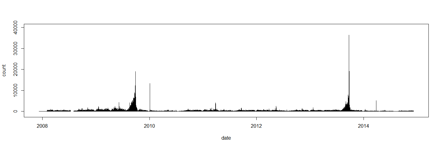
The public attention for the Wikipedia article peaks well above 35,000 views per day and overall we find two distinct bulks of attention, one in late 2009 and one in late 2013.
Tweaking the plot
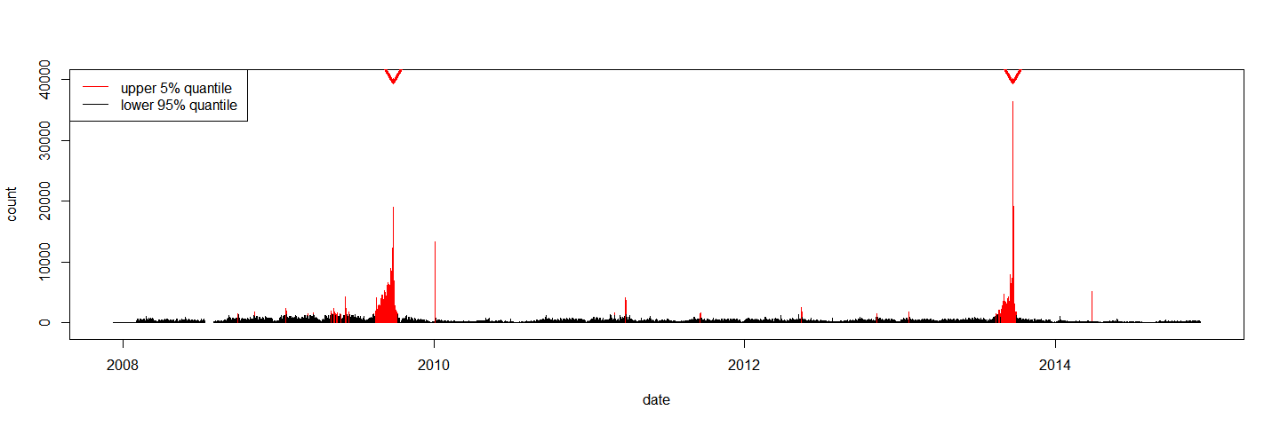
Let’s put some more effort into the visualization by splitting the counts into normals (lower 95% of the values) and those that are unusually large (upper 5% of the values).
count_big       <- bt_election$count > quantile(bt_election$count, 0.95)
count_big_col   <- ifelse(count_big, "red", "black")
The following command visualizes the page access counts for the Wikipedia article Bundestagswahl from the German Wikipedia on a daily basis with red bars for the upper 5% of the values and black bars for the remaining 95%. The triangles at the top of the figure mark the two election dates -- 27th of September in 2009 and 22nd of September in 2013.
plot(  bt_election,
       type = "h",
       col  = count_big_col,
       ylim = c(-1000,40000))
arrows( x0  = as.numeric(c(wp_date("2013-09-22"),wp_date("2009-09-27"))),
        x1  = as.numeric(c(wp_date("2013-09-22"),wp_date("2009-09-27"))),
        y0  = 40000,
        y1  = 39500,
        lwd = 3,
        col = "red")
legend( x     = "topleft",
        col   = c("red", "black"),
       legend = c("upper 5% quantile", "lower 95% quantile"),
       lwd    = 1)
Credits
Thanks go out to Domas Mituzas and User:Henrik for data and API provided at stats.grok.se.